Intended for healthcare professionals
Home/About BMJ/Resources for readers/Publications/Statistics at square one/6. Differences between percentages and paired alternatives
6. Differences between percentages and paired alternatives
Standard error of difference between percentages or proportions
The surgical registrar who investigated appendicitis cases, referred to in Chapter 3 , wonders whether the percentages of men and women in the sample differ from the percentages of all the other men and women aged 65 and over admitted to the surgical wards during the same period. After excluding his sample of appendicitis cases, so that they are not counted twice, he makes a rough estimate of the number of patients admitted in those 10 years and finds it to be about 12-13 000. He selects a systematic random sample of 640 patients, of whom 363 (56.7%) were women and 277 (43.3%) men.
The percentage of women in the appendicitis sample was 60.8% and differs from the percentage of women in the general surgical sample by 60.8 – 56.7 = 4.1%. Is this difference of any significance? In other words, could this have arisen by chance?
There are two ways of calculating the standard error of the difference between two percentages: one is based on the null hypothesis that the two groups come from the same population; the other on the alternative hypothesis that they are different. For Normally distributed variables these two are the same if the standard deviations are assumed to be the same, but in the binomial case the standard deviations depend on the estimates of the proportions, and so if these are different so are the standard deviations. Usually both methods give almost the same result.
Confidence interval for a difference in proportions or percentages
The calculation of the standard error of a difference in proportions p1 – p2 follows the same logic as the calculation of the standard error of two means; sum the squares of the individual standard errors and then take the square root. It is based on the alternative hypothesis that there is a real difference in proportions (further discussion on this point is given in Common questions at the end of this chapter).
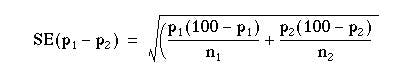
Note that this is an approximate formula; the exact one would use the population proportions rather than the sample estimates. With our appendicitis data we have:

Thus a 95% confidence interval for the difference in percentages is
4.1 – 1.96 x 4.87 to 4.1 + 1.96 x 4.87 = -5.4 to 13.6%.
Significance test for a difference in two proportions
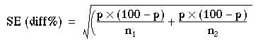
For a significance test we have to use a slightly different formula, based on the null hypothesis that both samples have a common population proportion, estimated by p.
To obtain p we must amalgamate the two samples and calculate the percentage of women in the two combined; 100 – p is then the percentage of men in the two combined. The numbers in each sample are  and
and  .
.
Number of women in the samples: 73 + 363 = 436
Number of people in the samples: 120 + 640 = 760
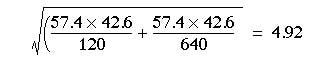
Percentage of women: (436 x 100)/760 = 57.4
Percentage of men: (324 x 100)/760 = 42.6
Putting these numbers in the formula, we find the standard error of the difference between the percentages is 4.1-1.96 x 4.87 to 4.1 + 1.96 x 4.87 = -5.4 to 13.6%
This is very close to the standard error estimated under the alternative hypothesis.
The difference between the percentage of women (and men) in the two samples was 4.1%. To find the probability attached to this difference we divide it by its standard error: z = 4.1/4.92 = 0.83. From Table A (Appendix table A.pdf) we find that P is about 0.4 and so the difference between the percentages in the two samples could have been due to chance alone, as might have been expected from the confidence interval. Note that this test gives results identical to those obtained by the  test without continuity correction (described in Chapter 7).
Standard error of a total
The total number of deaths in a town from a particular disease varies from year to year. If the population of the town or area where they occur is fairly large, say, some thousands, and provided that the deaths are independent of one another, the standard error of the number of deaths from a specified cause is given approximately by its square root,  Further, the standard error of the difference between two numbers of deaths, and , can be taken as
  .
.
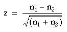
This can be used to estimate the significance of a difference between two totals by dividing the difference by its standard error:
 (6.1)
(6.1)It is important to note that the deaths must be independently caused; for example, they must not be the result of an epidemic such as influenza. The reports of the deaths must likewise be independent; for example, the criteria for diagnosis must be consistent from year to year and not suddenly change in accordance with a new fashion or test, and the population at risk must be the same size over the period of study.
In spite of its limitations this method has its uses. For instance, in Carlisle the number of deaths from ischaemic heart disease in 1973 was 276. Is this significantly higher than the total for 1972, which was 246? The difference is 30. The standard error of the difference is  . We then take z = 30/22.8 = 1.313. This is clearly much less than 1.96 times the standard error at the 5% level of probability. Reference to appendix-table.pdftable A shows that P = 0.2. The difference could therefore easily be a chance fluctuation.
This method should be regarded as giving no more than approximate but useful guidance, and is unlikely to be valid over a period of more than very few years owing to changes in diagnostic techniques. An extension of it to the study of paired alternatives follows.
Paired alternatives
Sometimes it is possible to record the results of treatment or some sort of test or investigation as one of two alternatives. For instance, two treatments or tests might be carried out on pairs obtained by matching individuals chosen by random sampling, or the pairs might consist of successive treatments of the same individual (see Chapter 7 for a comparison of pairs by the tt test). The result might then be recorded as “responded or did not respond”, “improved or did not improve”, “positive or negative”, and so on. This type of study yields results that can be set out as shown in table 6.1.
Table 6.1
| Member of pair receiving treatment A | Member of pair receiving treatment B |
|---|---|
| Responded | Responded (1) |
| Responded | Did not respond (2) |
| Did not respond | Responded (3) |
| Did not respond | Did not respond (2) |
The significance of the results can then be simply tested by McNemar’s test in the following way. Ignore rows (1) and (4), and examine rows (2) and (3). Let the larger number of pairs in either of rows (2) or (3) be called n1 and the smaller number of pairs in either of those two rows be n2. We may then use formula ( 6.1 ) to obtain the result, z. This is approximately Normally distributed under the null hypothesis, and its probability can be read from appendix-table.pdftable A.
However, in practice, the fairly small numbers that form the subject of this type of investigation make a correction advisable. We therefore diminish the difference between n1and n2 by using the following formula:
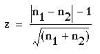
where the vertical lines mean “take the absolute value”.
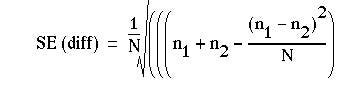
Again, the result is Normally distributed, and its probability can be read from. As for the unpaired case, there is a slightly different formula for the standard error used to calculate the confidence interval.(1) Suppose N is the total number of pairs, then
For example, a registrar in the gastroenterological unit of a large hospital in an industrial city sees a considerable number of patients with severe recurrent aphthous ulcer of the mouth. Claims have been made that a recently introduced preparation stops the pain of these ulcers and promotes quicker healing than existing preparations.
Over a period of 6 months the registrar selected every patient with this disorder and paired them off as far as possible by reference to age, sex, and frequency of ulceration. Finally she had 108 patients in 54 pairs. To one member of each pair, chosen by the toss of a coin, she gave treatment A, which she and her colleagues in the unit had hitherto regarded as the best; to the other member she gave the new treatment, B. Both forms of treatment are local applications, and they cannot be made to look alike. Consequently to avoid bias in the assessment of the results a colleague recorded the results of treatment without knowing which patient in each pair had which treatment. The results are shown in Table 6.2
| Member of pair receiving treatment A | Member of pair receiving treatment B | Pairs of patients |
|---|---|---|
| Responded | Responded | 16 |
| Responded | Did not respond | 23 |
| Did not respond | Responded | 10 |
| Did not respond | Did not respond | 5 |
| Total | 54 |
Here n1=23, n2=10. Entering these values in formula (6.1) we obtain
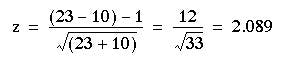
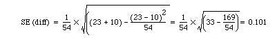
The probability value associated with 2.089 is about 0.04 Table A. Therefore we may conclude that treatment A gave significantly better results than treatment B. The standard error for the confidence interval is
23/54 – 10/54 = 0.241
The 95% confidence interval for the difference in proportions is
0.241 – 1.96 x 0.101 to 0.241 + 1.96 x 0.10 that is, 0.043 to 0.439.
0.241 – 1.96 x 0.101 to 0.241 + 1.96 x 0.10 that is, 0.043 to 0.439.
Although this does not include zero, the confidence interval is quite wide, reflecting uncertainty as to the true difference because the sample size is small. An exact method is also available.
Common questions
Why is the standard error used for calculating a confidence interval for the difference in two proportions different from the standard error used for calculating the significance?
For nominal variables the standard deviation is not independent of the mean. If we suppose that a nominal variable simply takes the value 0 or 1, then the mean is simply the proportion of is and the standard deviation is directly dependent on the mean, being largest when the mean is 0.5. The null and alternative hypotheses are hypotheses about means, either that they are the same (null) or different (alternative). Thus for nominal variables the standard deviations (and thus the standard errors) will also be different for the null and alternative hypotheses. For a confidence interval, the alternative hypothesis is assumed to be true, whereas for a significance test the null hypothesis is assumed to be true. In general the difference in the values of the two methods of calculating the standard errors is likely to be small, and use of either would lead to the same inferences. The reason this is mentioned here is that there is a close connection between the test of significance described in this chapter and the Chi square test described in Chapter 8. The difference in the arithmetic for the significance test, and that for calculating the confidence interval, could lead some readers to believe that they are unrelated, whereas in fact they are complementary. The problem does not arise with continuous variables, where the standard deviation is usually assumed independent of the mean, and is also assumed to be the same value under both the null and alternative hypotheses.
It is worth pointing out that the formula for calculating the standard error of an estimate is not necessarily unique: it depends on underlying assumptions, and so different assumptions or study designs will lead to different estimates for standard errors for data sets that might be numerically identical.
References
1. Gardner MJ, Altman DG, editors. Statistics with Confidence. London: BMJ Publishing, 1989:31.
Exercises
Exercise 6.1
In an obstetric hospital l7.8% of 320 women were delivered by forceps in 1975. What is the standard error of this percentage? In another hospital in the same region 21.2% of 185 women were delivered by forceps. What is the standard error of the difference between the percentages at this hospital and the first? What is the difference between these percentages of forceps delivery with a 95% confidence interval and what is its significance?
Exercise 6.2
A dermatologist tested a new topical application for the treatment of psoriasis on 47 patients. He applied it to the lesions on one part of the patient’s body and what he considered to be the best traditional remedy to the lesions on another but comparable part of the body, the choice of area being made by the toss of a coin. In three patients both areas of psoriasis responded; in 28 patients the disease responded to the traditional remedy but hardly or not at all to the new one; in 13 it responded to the new one but hardly or not at all to the traditional remedy; and in four cases neither remedy caused an appreciable response. Did either remedy cause a significantly better response than the other?